IBM6520 Group Project - Coffee Vending

Authors

Affiliation

Min Gong

Cal Poly Pomona

Jarrod Griffin

Cal Poly Pomona

Ceren Unal

Cal Poly Pomona

Eunice Won

Cal Poly Pomona

Published

May 12, 2025

Important

Live Version Here: Click here to view a live web version of this document.

Presentation Here: Click here to view the accompanying presentation version.

Introduction

Effective inventory control for coffee-vending machines hinges on anticipating weekly ingredient consumption while avoiding costly spoilage. We forecast demand using historical sales from two machines, delivering eight-week projections that guide stock levels and reorder cadence.

This report:

Imports & cleans transaction data from a coffee vending machine.
Explores key demand drivers.
Models weekly sales with Seasonal ARIMA.
Delivers eight-week forecasts and stocking recommendations.

Executive Summary with Actionable Recommendations

Executive Summary

This report delivers an integrated forecasting solution for a coffee vending machine using transaction data from March 2024 to March 2025. We modeled the trends in ingredient usage, coffee type unit sales, and overall revenue to generate eight-week forecasts that guide more precise inventory management and restocking decisions.

Ingredient Usage: From the EDA, we can see that milk is the most volatile and heavily used ingredient, peaking at over 16,000mL in some weeks due to high demand for milk-based drinks. Coffee grounds remain stable, while the usage of chocolate and sugar show seasonal spikes. The seasonal spikes may be due to the cold weather and consumers preferring hot drinks, like hot chocolate and cocoa.

Seasonal ARIMA models effectively captured ingredient usage patterns, with Ljung-Box tests confirming white-noise residuals. All ingredient seasonal ARIMA models have uncorrelated residuals and is reliable for forecasting.
Drink Sales Patterns: Americano with Milk and Latte was seen as the most popular and consistently sold drinks. Cortado and Espresso was seen to be less popular in sales and could be reconsidered for prioritization.
Revenue Trends: Weekly revenue fluctuates and showed peaks that resembled “three hills”. The STL decomposition showed a trend, but it did not show significant seasonality. The ETS model projects stable short-term growth.

For forecasting, we used two different methods: ARIMA for coffee types and ETS for revenue. The ARIMA model was used to automatically difference the data and then revert forecasts to the original scale, enabling predictions of unit sales over time. The model indicates that sales will remain mostly stable over the next eight weeks, though cortado, latte, and hot chocolate may see slight declines, suggesting a potential need to reduce their production and packaging. The ETS model, which emphasizes recent trends, forecasts stable overall revenue during this period. We opted for ETS to generate a more robust model based on the trend with increasing periodic variance. Since we are forecasting for a short period (8 weeks) for higher accuracy, we don’t see the model capturing the upwards trend throughout the year.

Actionable Recommendations

Focus on High-Selling Drinks: Focus inventory on Americano with Milk and Latte ingredients to meet ongoing high sales volume. Make sure that there is an uninterrupted ingredient supply for the high-selling drinks.
Prioritize Milk Inventory: Proactively stock milk with a buffer margin, especially during high-consumption weeks to avoid any out-of-stock situations.
Deprioritize Low-Selling Drinks: Reevaluate stocking strategy for lower-selling drinks to minimize unnecessary ingredient usage. Can consider rotating low-selling drinks to optimize machine space and ingredient turnover.
Prepare for Seasonal Demand Spikes: Slightly increase sugar and chocolate inventory in colder months or during promotional periods when the demand for hot drinks increase.
Automate Coffee Reorders: Use consistent SARIMA forecasts to consider setting up auto-reordering for coffee grounds and to avoid overstocking.
Update Forecast Models Regularly: Update forecast models regularly to see the changes in trend and seasonality and to take that into effect. Update SARIMA and ETS models quarterly to reflect changes in customer behavior or seasonal effects.

Data and Assumptions

Kaggle data is from two vending machines. Below we will import the two datasets and combine them.

Raw Transaction Data

Transaction data was taken from the following Kaggle link:

https://www.kaggle.com/datasets/ihelon/coffee-sales

Code

machine1 <- read_csv("data/index_1.csv") %>% 
  mutate(machine_id = "machine1")

sales <- machine1 |>
  mutate(date = as_date(date),
         datetime = as_datetime(datetime),
         coffee_name=toupper(coffee_name))

Products and Ingredients

In the dataset, only product names are given. In order to more accurately predict what ingredients are needed and when, we must decompose the product into its ingredients. See below for the assumptions made for each of the 8 unique products.

Unique Products

Code

unique(sales$coffee_name)%>%sort()

[1] "AMERICANO"           "AMERICANO WITH MILK" "CAPPUCCINO"         
[4] "COCOA"               "CORTADO"             "ESPRESSO"           
[7] "HOT CHOCOLATE"       "LATTE"

Ingredients

Code

recipes <- tribble(
  ~coffee_name,            ~coffeeG, ~milkML, ~chocolateG,  ~sugarG, ~vanillaML,
  "AMERICANO",                18,       0,          0,         0,        0,
  "AMERICANO WITH MILK",      18,      60,          0,         0,        0,
  "CAPPUCCINO",               18,     100,          0,         0,        0,
  "COCOA",                     0,     240,         22,        15,        0,
  "CORTADO",                  18,      60,          0,         0,        0,
  "ESPRESSO",                 18,       0,          0,         0,        0,
  "HOT CHOCOLATE",             0,     240,         30,        20,        0,
  "LATTE",                    18,     240,          0,         0,       10
)

Ingredient Logic

Drink	Ingredient-logic rationale
Espresso	Straight double shot: 18 g ground coffee, no additives (Specialty Coffee Association 2018).
Americano	Same 18 g espresso diluted with ≈ 4 × its volume of hot water; nothing else required (Specialty Coffee Association 2018).
Americano with Milk	Americano softened with ≈ 60 ml steamed milk – enough to mellow bitterness without turning it into a latte (Cordell 2024).
Cappuccino	Classic 1 : 1 : 1 build – espresso, ≈ 60 ml steamed milk, equal micro-foam – fills a 150–180 ml cup (Raffii 2024).
Cortado	Spanish “cut” drink: equal parts double espresso and ≈ 60 ml steamed milk (Wine Editors 2025).
Latte	U.S. latte stretches the shot with ≈ 240 ml milk (1 : 4–5 ratio); vanilla version adds 10 ml syrup (≈ 2 pumps) (Coffee Bros. 2024; Page 2025).
Cocoa	Non-coffee mix: 240 ml milk + 22 g cocoa powder + 15 g sugar – standard stovetop proportions (Hersheyland Test Kitchen 2025).
Hot Chocolate	Richer café blend: same milk but 30 g cocoa and 20 g sugar for modern sweetness level (Hersheyland Test Kitchen 2025).

Combining Transaction Data and Recipies

Below we will join the two tables on the coffee name, which will add ingredients to all rows in the transaction data. Explore the data we will use in our analysis below:

Code

sales_ingredients <- sales |>
  left_join(recipes, by = "coffee_name") |>
  replace_na(list(
    coffeeG = 0, milkML = 0, chocolateG = 0, sugarG = 0, vanillaML = 0
  ))

Converting to Weekly Series

We aggregate to a weekly time series because the business decisions we are informing, like re-ordering coffee, milk, chocolate, etc, are made on a weekly cadence. Collapsing daily transactions into weeks smooths out erratic, day-to-day swings leaving a cleaner signal that aligns directly with the quantity we must predict.

We will also convert to a time series type object and verify it has no gaps in the series. If we see FALSE from .gaps, then we have no gaps.

Code

weekly_sales <- sales_ingredients |>
  mutate(week = lubridate::floor_date(date, unit = "week")) |>
  group_by(week) |>
  summarise(across(coffeeG:vanillaML, sum, na.rm = TRUE),
            sales_n = n()) |>
  ungroup()

weekly_sales <- weekly_sales|>
  as_tsibble(index = week)

has_gaps(weekly_sales)

# A tibble: 1 × 1
  .gaps
  <lgl>
1 FALSE

Exploratory Insights (EDA)

Data Description & Exploratory Summary

Dataset Overview

This dataset is derived from the raw sales table and represents the total weekly revenue, aggregated across all transactions from coffee vending machines, covering the period from March 2024 to March 2025, with data on 8 types of coffee.

EDA Findings

The weekly revenue time series is complete with no missing weeks. The revenue exhibits a distinct trend, characterized by three major peaks, resembling a “three hills” pattern. STL decomposition confirmed a clear trend but did not detect significant seasonality. After first-order differencing, the series became stationary, with the ACF indicating white noise. The highest revenue occurred in the week of October 6, 2024, amounting to $3,546, while the lowest revenue was recorded in the week of March 23, 2025, at $204.76. The observed fluctuation pattern suggests that external drivers, such as promotions or demand cycles, may play a role.

Assumptions

Revenue can be modeled primarily as a trend-driven process, with the data-generating process in the next 8 weeks expected to mirror that of the recent 8 weeks. Weekly sales are projected to grow in the upcoming week, continuing the observed trend.

Code

#weekly revenue tsibble
weekly_revenue <- sales %>%
  mutate(week = floor_date(date, unit = "week")) %>%
  group_by(week) %>%
  summarise(total_revenue = sum(money, na.rm = TRUE), .groups = "drop") %>%
  as_tsibble(index = week)

Code

#Interactive weekly revenue
weekly_revenue %>%
  ggplot(aes(x = week, y = total_revenue)) +
  geom_line(color = "steelblue", size = 1.2) +
  labs(title = "Interactive Weekly Revenue",
       y = "Revenue ($)", x = NULL) +
  theme_minimal() -> p

ggplotly(p)

Code

#STL Decomposition
decomposed_revenue <- weekly_revenue %>%
  model(STL(total_revenue ~ season() + trend(), robust = TRUE)) %>%
  components()

# plot component
autoplot(decomposed_revenue) +
  labs(title = "STL Decomposition of Weekly Revenue",
       x = "Week", y = NULL) +
  theme_minimal()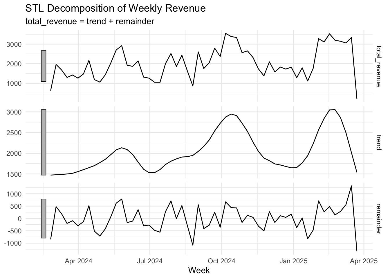

Code

#Differencing
diff_revenue <- weekly_revenue %>%
  mutate(diff_revenue = difference(total_revenue, lag = 1))  

autoplot(diff_revenue, diff_revenue) +
  labs(title = "First Difference of Weekly Revenue",
       y = "Differenced Revenue",
       x = "Week") +
  theme_minimal()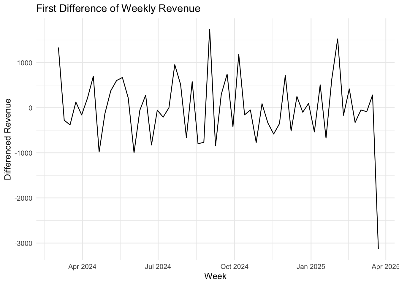

Code

# ACF
diff_revenue %>%
  ACF(diff_revenue, lag_max = 30) %>%
  autoplot() +
  labs(title = "ACF of Differenced Revenue")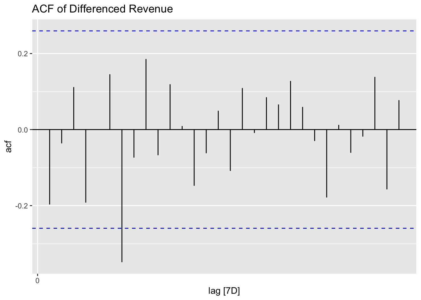

Code

# Summary stats
summary_stats <- weekly_revenue %>%
  summarise(
    mean_revenue = mean(total_revenue, na.rm = TRUE),
    median_revenue = median(total_revenue, na.rm = TRUE),
    max_revenue = max(total_revenue, na.rm = TRUE),
    min_revenue = min(total_revenue, na.rm = TRUE)
  )

# Highest Weekly Sales
top_week <- weekly_revenue %>%
  filter(total_revenue == max(total_revenue, na.rm = TRUE))
top_week

# A tsibble: 1 x 2 [7D]
  week       total_revenue
  <date>             <dbl>
1 2024-10-06         3547.

Code

datatable(summary_stats, caption = "Weekly Revenue Summary Stats")

Data Description & Exploratory Summary

Dataset Overview

This dataset represents the weekly sales volume (cups sold) for 8 different coffee types from March 2024 to March 2025.

EDA Findings

The dataset is mostly complete, with only a few missing values for certain coffee types in specific weeks. Among the weeks with over 30 cups sold, Americano appeared 5 times, Americano with Milk 2 times, and Latte 2 times. While gg_season() plots suggest that each coffee type exhibits weak seasonal patterns, the short time span of the data (approximately one year) was not enough for STL decomposition to confidently detect seasonality.

Assumptions

Americano with Milk is expected to remain the top-selling coffee over the next 8 weeks, continuing its strong performance observed historically. However, customer preferences may shift across coffee types due to changes in weather. Any growth patterns are likely to be gradual rather than abrupt, with no coffee type expected to suddenly double or halve in volume.

Code

#sales of each coffee type
weekly_coffee_volume <- sales %>%
  mutate(week = floor_date(date, unit = "week")) %>%
  group_by(week, coffee_name) %>%
  summarise(
    total_volume = n(),  
    .groups = "drop"
  ) %>%
  as_tsibble(index = week, key = coffee_name)

Code

# Weekly cups sold by coffee type
weekly_coffee_volume %>%
  autoplot(total_volume) +
  facet_wrap(~coffee_name, scales = "free_y") +
  labs(title = "Weekly Cups Sold by Coffee Type",
       y = "Number of Cups", x = "") +
  theme_minimal() +
  theme(axis.text.x = element_text(angle = 45, hjust = 1),
        legend.position = "none")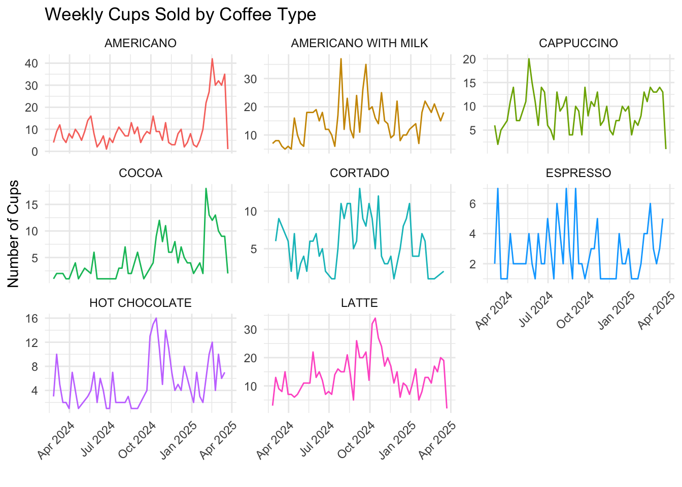

Code

# Check NA
missing_data <- weekly_coffee_volume %>%
  group_by(coffee_name) %>%
  summarise(missing_weeks = sum(is.na(total_volume)))


#fill gap
weekly_volume_filled <- weekly_coffee_volume %>%
  fill_gaps(total_volume = 0)

#gg_season
weekly_volume_filled%>%
  gg_season(total_volume) +
  facet_wrap(~ coffee_name, scales = "free_y") +
  labs(title = "Seasonal Plot of Weekly Coffee Volume",
       x = "Week of Year", y = "Total Volume") +
  theme_minimal()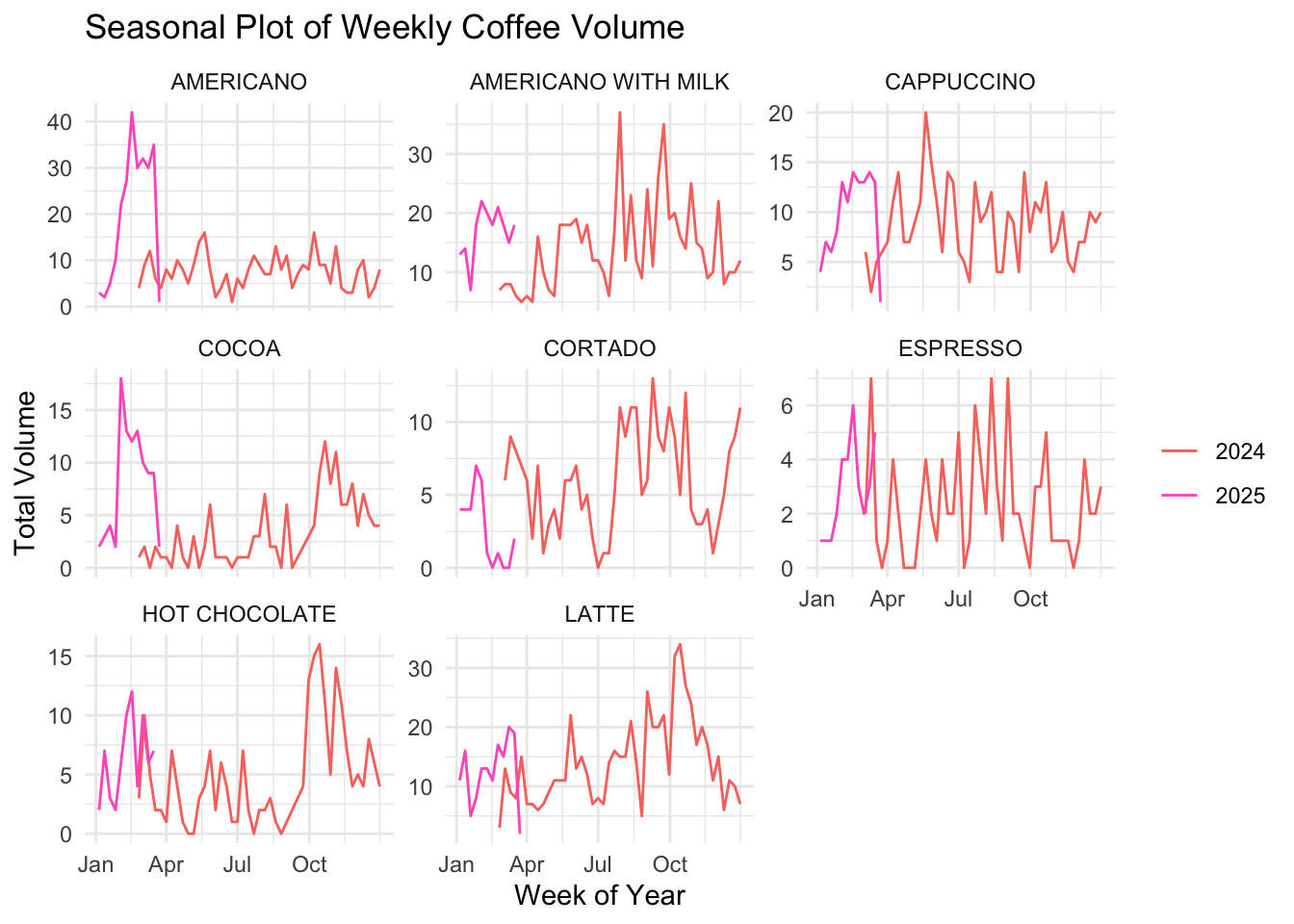

Code

#decomposition
decomposed_volume <- weekly_volume_filled %>%
  model(
    STL(total_volume ~ season(window = 52) + trend(window = 7), robust = TRUE)
  ) %>%
  components()

autoplot(decomposed_volume) +
  facet_wrap(~coffee_name, scales = "free_y") +
  labs(title = "STL Decomposition of Weekly Volume by Coffee Type",
       x = "Week", y = NULL) +
  theme_minimal() +
  theme(axis.text.x = element_text(angle = 45, hjust = 1),
        legend.position = "none")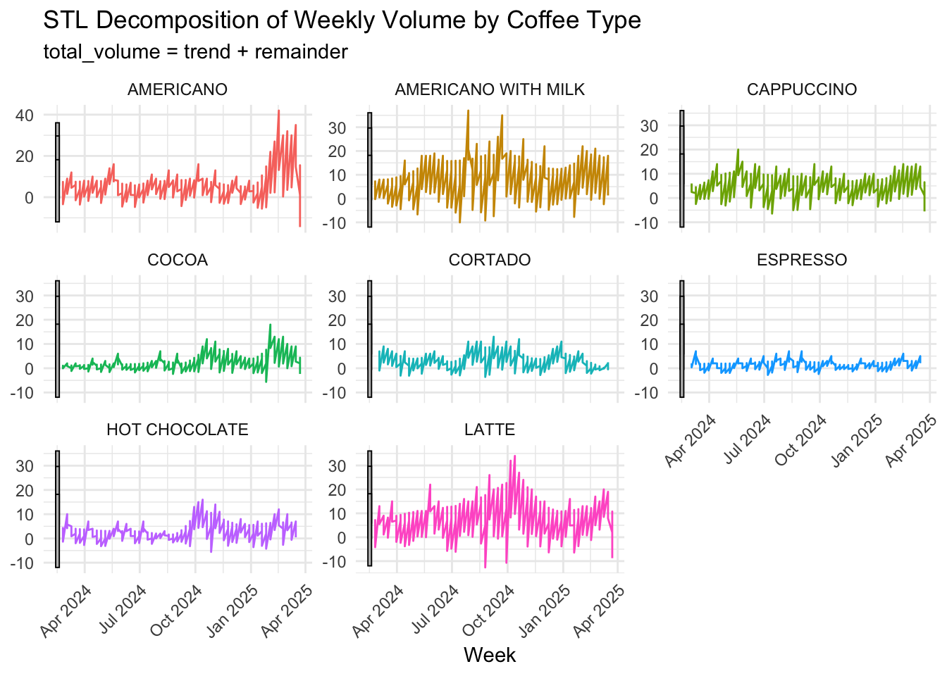

Code

#Differencing for all coffee type
weekly_volume_diff <- weekly_volume_filled %>%
  group_by(coffee_name) %>%
  mutate(diff_volume = difference(total_volume)) %>%
  ungroup()

Code

#tsibble：
weekly_volume_diff_tsibble <- weekly_volume_diff %>%
  filter(!is.na(diff_volume)) %>%
  as_tsibble(index = week, key = coffee_name)

# ACF
acf_diff_data <- weekly_volume_diff_tsibble %>%
  ACF(diff_volume)

#facet ACF 
acf_diff_data %>%
  autoplot() +
  facet_wrap(~ coffee_name, scales = "free_y") +
  labs(title = "ACF After Differencing (by Coffee Type)",
       x = "Lag", y = "ACF") +
  theme_minimal() +
  theme(axis.text.x = element_text(angle = 45, hjust = 1),
        legend.position = "none")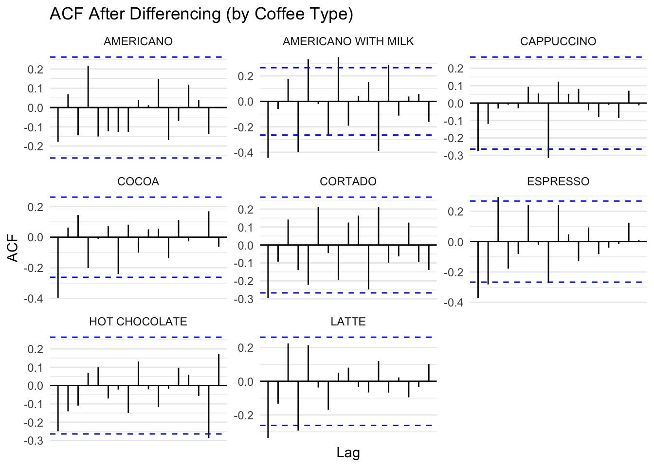

Code

coffee_summary <- weekly_coffee_volume %>%
  group_by(coffee_name) %>%
  summarise(
    total_cups = sum(total_volume, na.rm = TRUE),
    avg_weekly_cups = mean(total_volume, na.rm = TRUE),
    max_weekly_cups = max(total_volume, na.rm = TRUE),
    week_of_max_sales = week[which.max(total_volume)],
    min_weekly_cups = min(total_volume, na.rm = TRUE),
    week_of_min_sales = week[which.min(total_volume)],
    .groups = "drop"
  ) %>%
  mutate(
    percent_of_total = total_cups / sum(total_cups) * 100
  ) %>%
  arrange(desc(total_cups))  

datatable(coffee_summary,
          caption = "Coffee Type Weekly Sales Summary",
          options = list(pageLength = 8, scrollX = TRUE),
          rownames = FALSE) %>%
  formatRound(columns = c("avg_weekly_cups", "percent_of_total"), digits = 2)

Data Description & Exploratory Summary

Dataset Overview

This dataset represents weekly ingredient usage for a coffee vending machines from March 2024 to March 2025, including key ingredients like milk, coffee, chocolate, sugar, and vanilla.

EDA Findings

Among all ingredients, milk usage exhibits the highest variation and fluctuation, particularly evident in the STL decomposition. As the ingredient with the highest demand, milk also demonstrates significant volatility in its weekly usage. In contrast, other ingredients like coffee and chocolate show more stable, stationary patterns, with coffee being the second most demanded ingredient, displaying only slight fluctuations over time. Although the STL decomposition did not reveal clear seasonal components, the gg_season() plots suggest that some ingredients may have weak seasonal patterns. This discrepancy arises because STL decomposition typically requires at least two full seasonal cycles to robustly detect seasonality, while our dataset spans only around one year. Therefore, while statistical methods may not identify strong seasonal trends, visual tools like gg_season() remain valuable for uncovering subtle, recurring usage patterns across weeks of the year.

Assumptions

Given that milk consistently demonstrates the highest demand, it is reasonable to expect that it will remain the most used ingredient over the next 8 weeks. Meanwhile, ingredients such as coffee and chocolate are likely to maintain stable usage patterns, with only minor fluctuations potentially arising from consumer trends or specific events.

Code

# Weekly Ingredient Usage visualization
weekly_long %>%
  filter(metric != "sales_n") %>% 
  autoplot(value) +
  facet_wrap(~metric, scales = "free_y") +
  labs(title = "Weekly Ingredient Usage",
       y = "Amount Used",
       x = "") +
  theme_minimal() +
  theme(axis.text.x = element_text(angle = 45, hjust = 1),
        legend.position = "none")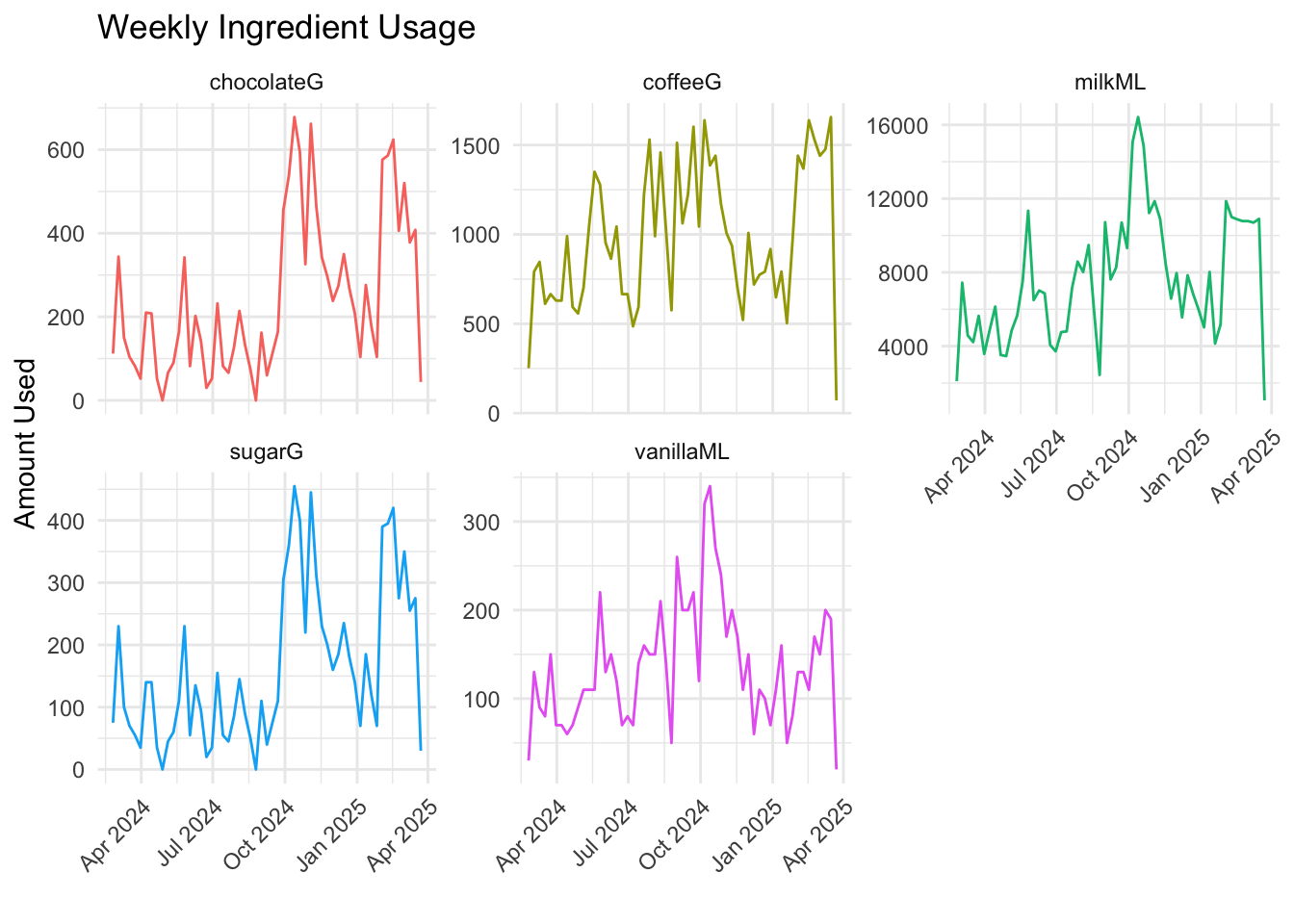

Code

#STL decomposition
decomp_recipe <- weekly_long %>%
  filter(metric != "sales_n") %>%
  model(
    STL(value ~ trend(window = 7), robust = TRUE)
  ) %>%
  components()

autoplot(decomp_recipe) +
  facet_wrap(~metric, scales = "free_y") +
  labs(title = "STL Decomposition of Ingredient Usage") +
  theme_minimal() +
  theme(legend.position = "none")+
  theme(axis.text.x = element_text(angle = 45, hjust = 1))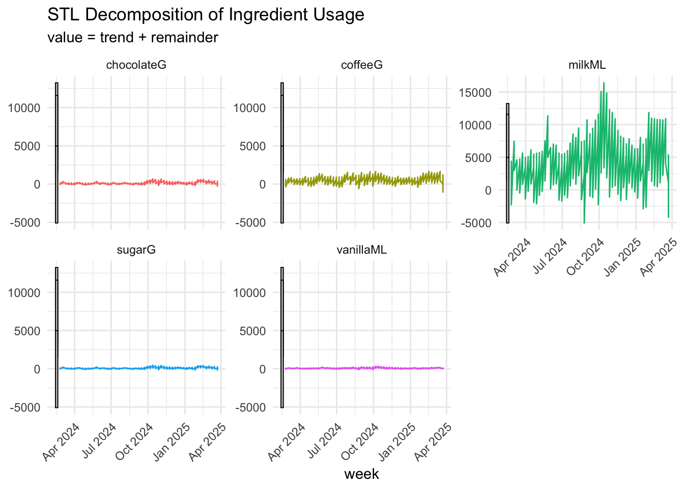

Code

#  gg_season to check seasonal pattern
gg_season(weekly_long, value) +
  facet_wrap(~ metric, scales = "free_y") +
  labs(title = "Seasonal Plot by Ingredient",
       x = "Week within Year", y = "Value") +
  theme_minimal()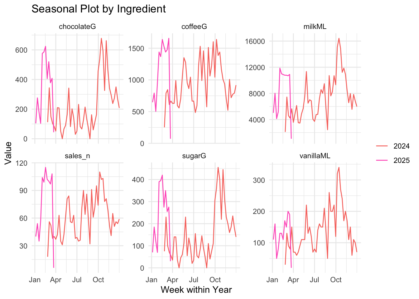

Code

#differencing
diff_recipe <- weekly_long %>%
  filter(metric != "sales_n") %>%
  mutate(diff_value = difference(value))

diff_recipe %>%
  autoplot(diff_value) +
  facet_wrap(~metric, scales = "free_y") +
  labs(title = "First-Order Differenced Ingredient Usage") +
  theme_minimal() +
  theme(axis.text.x = element_text(angle = 45, hjust = 1))+
  theme(legend.position = "none")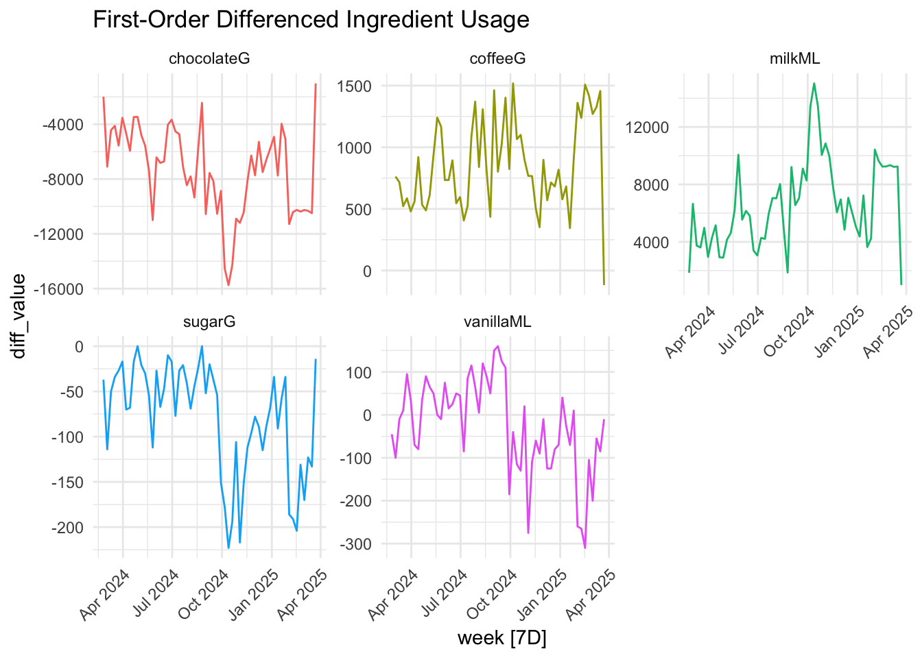

Code

#ACF 
diff_recipe %>%
  filter(!is.na(diff_value)) %>%
  ACF(diff_value) %>%
  autoplot() +
  facet_wrap(~metric, scales = "free_y") +
  labs(title = "ACF of First-Order Differenced Ingredient Usage") +
  theme_minimal()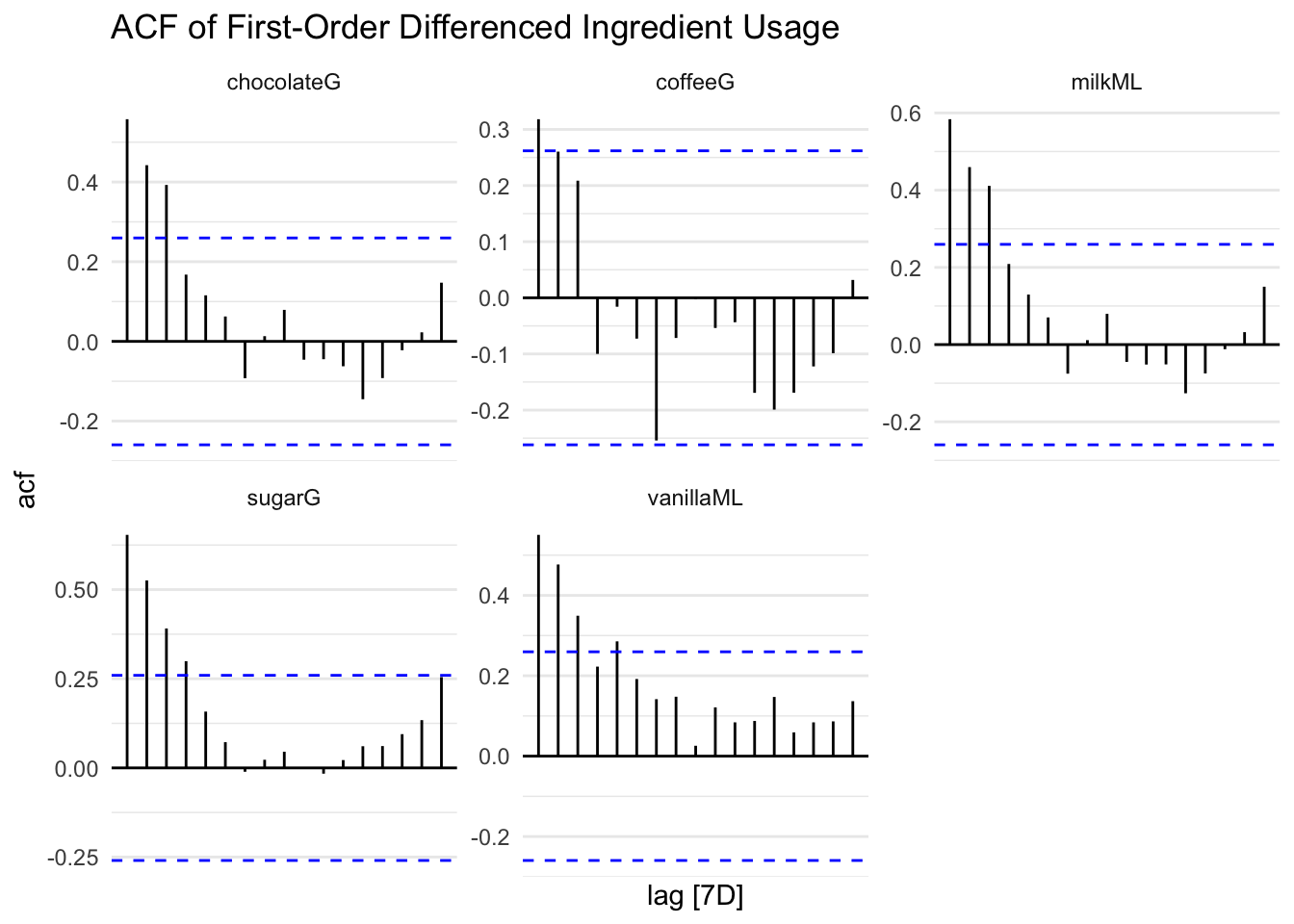

Code

ingredient_summary <- weekly_long %>%
  filter(metric != "sales_n") %>% 
  group_by(metric) %>%
  summarise(
    avg_weekly_usage = mean(value, na.rm = TRUE),
    min_weekly_usage = min(value, na.rm = TRUE),
    max_weekly_usage = max(value, na.rm = TRUE),
    total_usage = sum(value, na.rm = TRUE),
    weeks_count = n()
  ) %>%
  arrange(desc(avg_weekly_usage))

ingredient_summary

# A tsibble: 285 x 7 [7D]
# Key:       metric [5]
   metric week       avg_weekly_usage min_weekly_usage max_weekly_usage
   <chr>  <date>                <dbl>            <dbl>            <dbl>
 1 milkML 2024-10-13            16420            16420            16420
 2 milkML 2024-10-06            15080            15080            15080
 3 milkML 2024-10-20            14860            14860            14860
 4 milkML 2024-11-03            11860            11860            11860
 5 milkML 2025-02-02            11860            11860            11860
 6 milkML 2024-05-26            11340            11340            11340
 7 milkML 2024-10-27            11220            11220            11220
 8 milkML 2025-02-09            11000            11000            11000
 9 milkML 2024-11-10            10900            10900            10900
10 milkML 2025-03-16            10900            10900            10900
# ℹ 275 more rows
# ℹ 2 more variables: total_usage <dbl>, weeks_count <int>

Modeling Method Choice and Diagnostics

We model each weekly ingredient time series using Seasonal ARIMA (SARIMA), selected for its ability to capture both autoregressive and seasonal dynamics that is present in our exploratory data analysis. We want to produce stable 8-week forecasts to inform weekly inventory restocking decisions.

We first examine each ingredient’s stationarity and structure. After confirming data quality and transformation needs, we fit ARIMA models with seasonal terms. The March 23, 2025 week is excluded due to incomplete data.

Code

# Reshaping to time series per ingredient
ingredients <- c("coffeeG", "milkML", "chocolateG", "sugarG", "vanillaML")

ingredient_ts <- weekly_sales %>%
  select(week, coffeeG, milkML, chocolateG, sugarG, vanillaML) %>%
  pivot_longer(-week, names_to = "ingredient", values_to = "amount") %>%
  as_tsibble(index = week, key = ingredient)

Code

# Exclude March 23, 2025
ingredient_ts_filtered <- ingredient_ts %>%
  filter(week != "2025-03-23")

Code

# Long format tsibble
weekly_long_ingredients <- weekly_sales %>%
  pivot_longer(cols = coffeeG:vanillaML, names_to = "ingredient", values_to = "value") %>%
  as_tsibble(index = week, key = ingredient)

Code

# Fitting ARIMA to each ingredient using key grouping
ingredient_models <- weekly_long_ingredients %>%
  model(ARIMA(value))

# Fitting Seasonal ARIMA (SARIMA) to each ingredient series
arima_models <- ingredient_ts %>%
  model(ARIMA(value))

Model Evaluation and Diagnostics

For each ingredient, we examined residual plots from SARIMA to assess randomness, autocorrelation, and normality.

The Ljung-Box test results shown below evaluate whether the residuals from the ARIMA models are uncorrelated. It shows if the model has sufficiently captured all patterns in the time series.

Code

# Check residuals
ingredient_models %>%
  augment() %>%
  features(.resid, ljung_box, lag = 8) %>%
  datatable(caption = "Ljung-Box Test Results for Ingredient ARIMA Residuals")

Since the p-value is for all ingredients are greater than 0.05 (p > 0.05), there is no significant autocorrelation in residuals. This means that the model is adequate and that the residuals resembles white noise. All ingredient SARIMA models have uncorrelated residuals and can be confidently used for forecasting.

We may forecast coffee sales in two different ways: The unit sales forecast and change in unit sales forecast.

As the week of March 23 is incomplete and therefore, causes a sharp drop in revenue, we will be excluding that week from our models.

With differencing (Model forecasting change)

Having made most of our weekly coffee sales data set stationary after differencing once, we use ARIMA to create our model.

Code

#model with differencing
coffee_type_models_diff <- weekly_volume_diff %>%
  filter(coffee_name != "AMERICANO WITH MILK",
         week != "2025-03-23") %>%
  model(ARIMA(diff_volume))

We difference “Americano with Milk” coffee type a second time as differencing it once did not fix autocorrelation.

Code

americano_milk_diff <- weekly_volume_diff %>%
  filter(coffee_name == "AMERICANO WITH MILK",
         week != "2025-03-23") %>%
  mutate(diff_volume = difference(total_volume, differences = 2))

americano_milk_models_diff <- americano_milk_diff %>%
  model(ARIMA(diff_volume))

No differencing (Model forecasting unit sales)

Code

#model without differencing

coffee_type_models <- weekly_volume_diff %>%
  filter(week != "2025-03-23") %>%
  model(ARIMA(total_volume))

Due to the significant trend with increasing variance, we use ETS to train the revenue model. This model does not require differencing.

As the week of March 23 is incomplete and therefore, causes a sharp drop in revenue, we will be excluding that week from our model.

Code

revenue_models <- weekly_revenue %>%
  filter(week != "2025-03-23")  %>%
  model(ETS(total_revenue))

Generate Forecasts Results

Code

forecast_ingredients <- ingredient_models %>%
  forecast(h = "8 weeks")

autoplot(forecast_ingredients, weekly_long_ingredients) +
   labs(title = "8-Week Ingredient Forecasts (Seasonal ARIMA)",
       y = "Amount", x = "Week") +
  facet_wrap(~ingredient, scales = "free_y") +
  theme_minimal()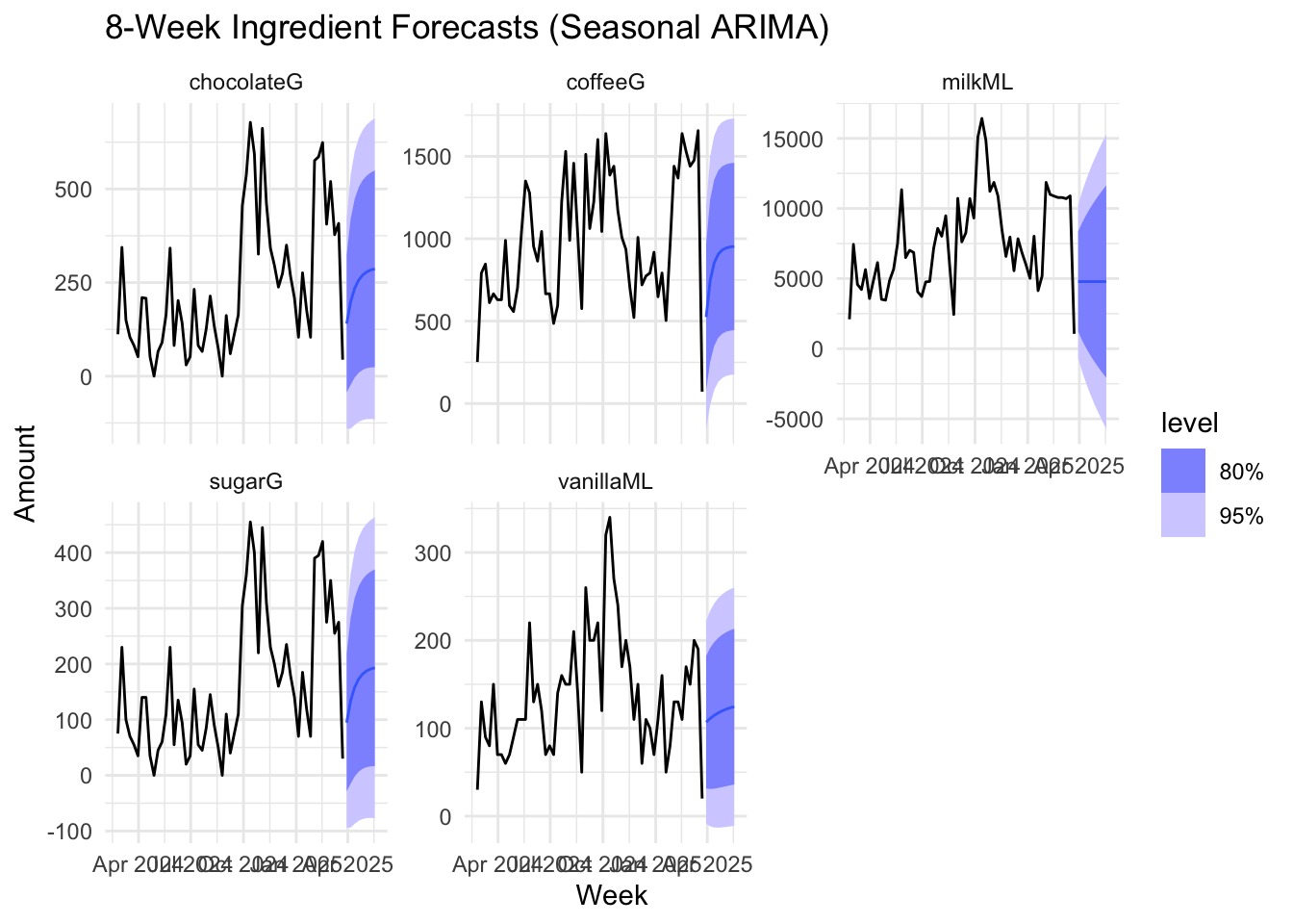

With differencing (Model forecasting change)

When forecasting differenced time series, we predict w much sales will change over time, not sales themselves. For most coffee types the ARIMA model expects those changes to average around zero.

Code

forecast_coffee_type_diff <- coffee_type_models_diff %>%
  forecast(h = "8 weeks")

autoplot(forecast_coffee_type_diff, weekly_volume_diff) +
   labs(title = "8-Week Coffee Type Forecasts (ARIMA)",
        subtitle = "1 Difference",
       y = "Amount", x = "Week") +
  facet_wrap(~coffee_name, scales = "free_y") +
  theme_minimal()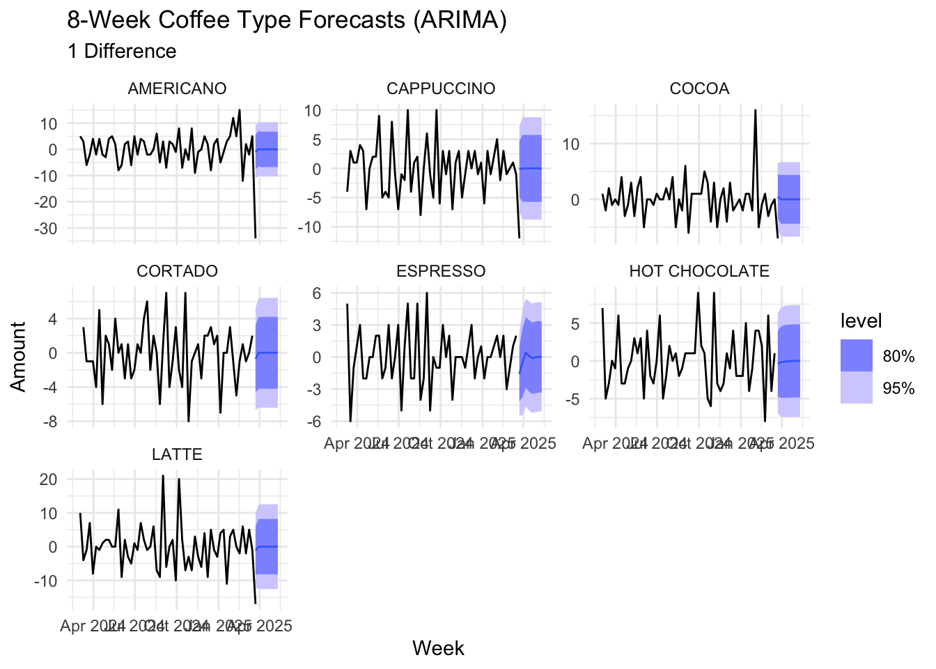

Americano with Milk - Forecast (2 Difference)

To remove autocorrelation, “americano with milk” coffee type was differenced twice. The ARIMA model predicts changes around zero, albeit with more fluctuation compared to other coffee types.

Code

forecast_americano_milk <- americano_milk_models_diff %>%
  forecast(h = "8 weeks")

autoplot(forecast_americano_milk, americano_milk_diff) +
   labs(title = "8-Week Americano With Milk Forecast (ARIMA)",
        subtitle = "2 Difference",
       y = "Amount", x = "Week") +
  facet_wrap(~coffee_name, scales = "free_y") +
  theme_minimal()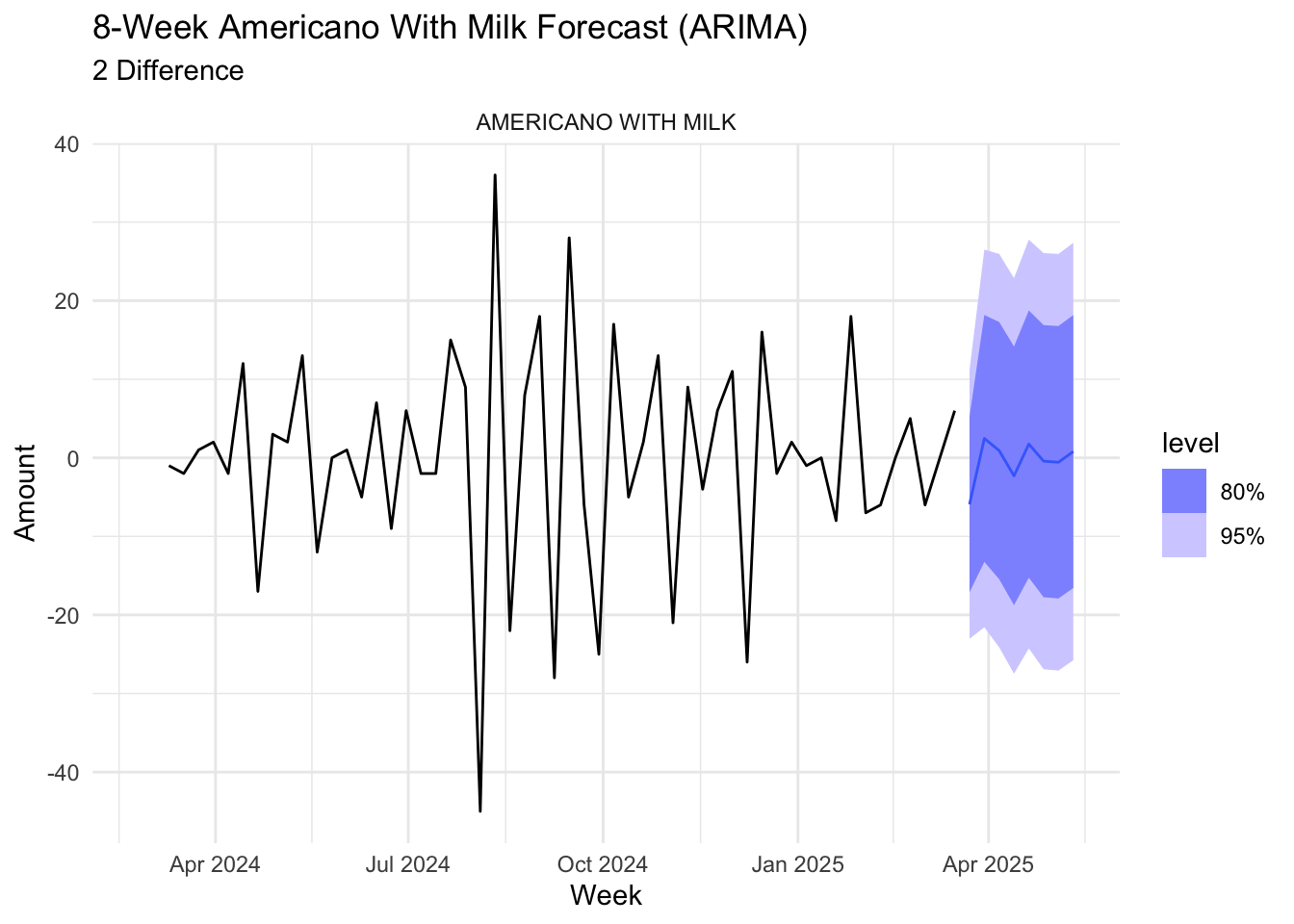

No differencing (Model forecasting unit sales)

Forecasting without differencing manually lets ARIMA do the differecning automatically and then revert the forecast back to the original scale, allowing us to forecast unit sales over time.

As the differenced ARIMA model suggests, the sales are expected to be relatively stable for most coffee types over the next 8 weeks. Cortado, latte and hot chocolate may see some decrease in sales. We should plan to decrease supply for those.

Code

forecast_coffee_type <- coffee_type_models %>%
  forecast(h = "8 weeks")

autoplot(forecast_coffee_type, weekly_volume_diff) +
   labs(title = "8-Week Coffee Type Forecasts (ARIMA)",
        subtitle = "No Differencing",
       y = "Amount", x = "Week") +
  facet_wrap(~coffee_name, scales = "free_y") +
  theme_minimal()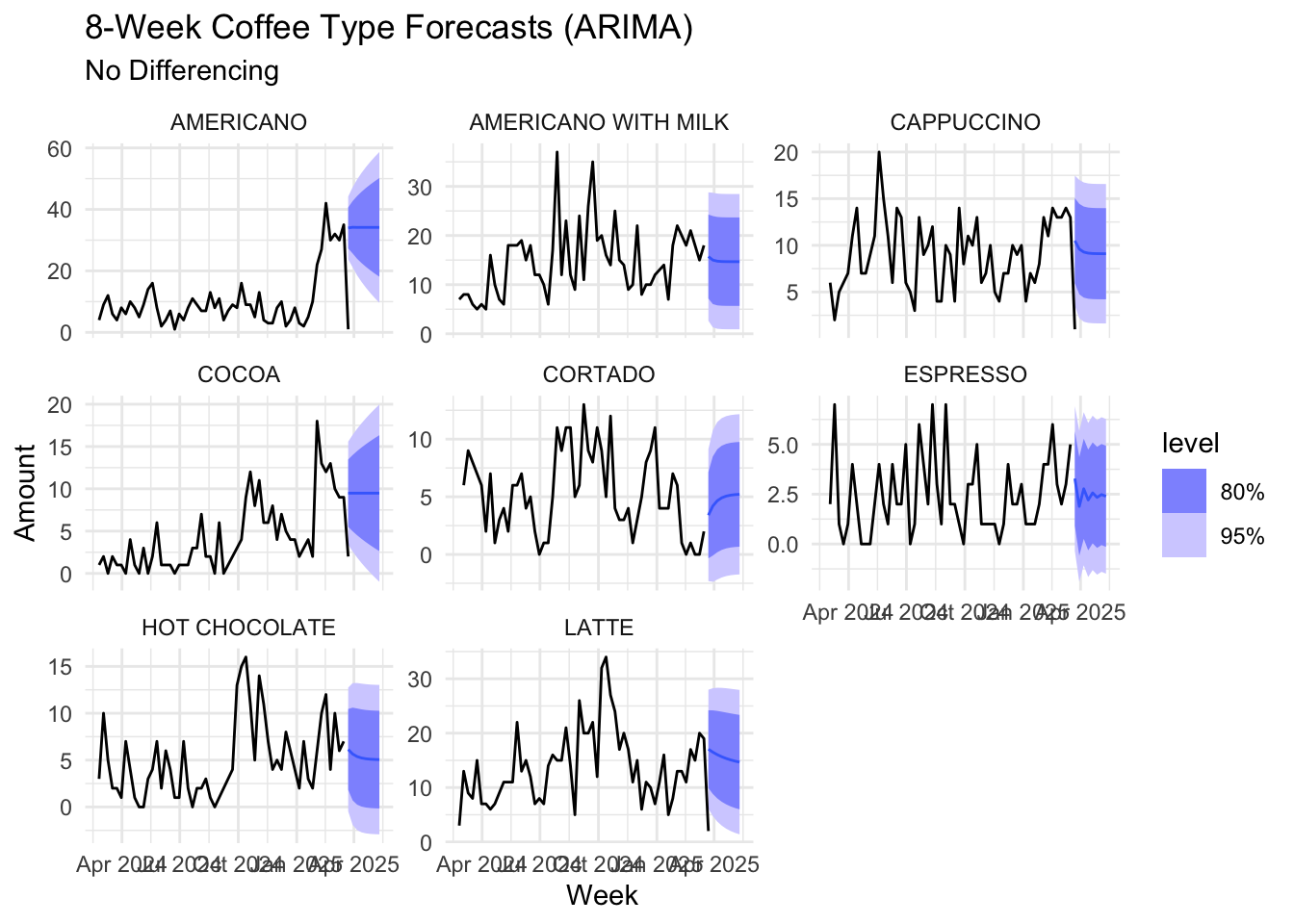

Given ETS, places more significance onto recent values, the forecasts predicts the revenue will be stable over the next 8 weeks.

Since the week of March 23 was incomplete, it was excluded from model training. As a result, while the current data (black line) show the weekly revenue around $300, the model predicts it will rise to $3000 by the end of the week based on the previous period.

Code

forecast_revenue <- revenue_models %>%
  forecast(h = "8 weeks")

autoplot(forecast_revenue, weekly_revenue) +
   labs(title = "8-Week Revenue Forecast (ETS)",
       y = "USD", x = "Week") +
  theme_minimal()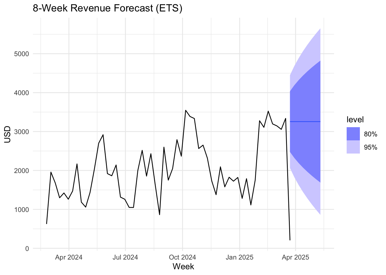

Conclusion

By using this report in aligning weekly inventory decisions with the forecasts, the coffee vending machine can reduce waste, maintain product availability, and improve cost-efficiency. This ensures customers to consistently find their preferred drinks stocked and ready.

Bonus After-Presentation Vector Autoregression (VAR)

Code

var_data <- weekly_sales %>%
  as.data.frame() %>%
  dplyr::select(coffeeG, milkML, chocolateG, sugarG, vanillaML) %>%
  tidyr::drop_na()

var_ts <- ts(var_data, frequency = 52)
var_model <- vars::VAR(var_ts, type = "const", lag.max = 8, ic = "AIC")
var_fc <- predict(var_model, n.ahead = 8)
plot(var_fc)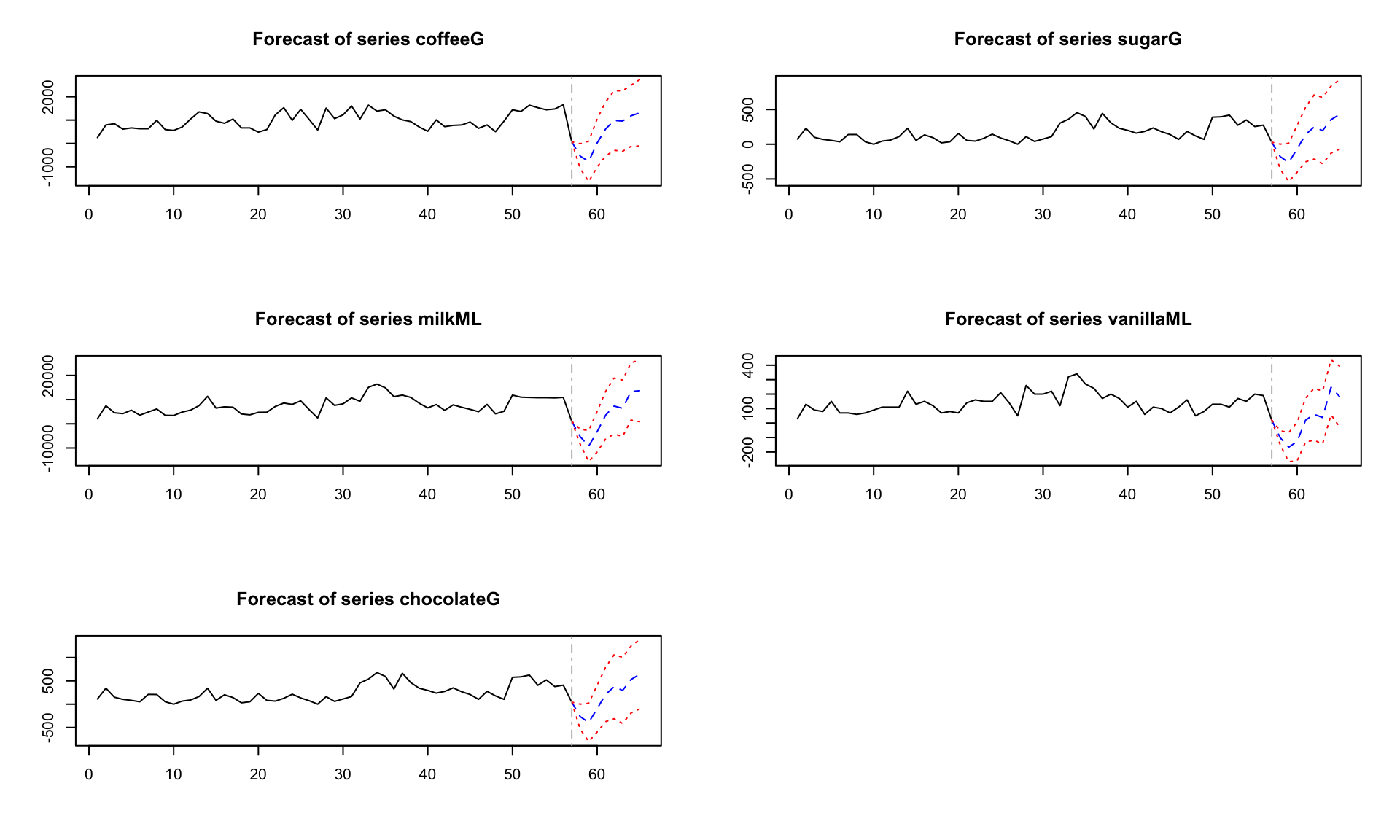

Code

# Calculate weekly ingredient usage per coffee type
weekly_ingredient_by_drink <- sales_ingredients %>%
  mutate(week = floor_date(date, unit = "week")) %>%
  group_by(week, coffee_name) %>%
  summarise(across(c(coffeeG, milkML, chocolateG, sugarG, vanillaML), sum, na.rm = TRUE),
            .groups = "drop")

weekly_ingredient_props <- weekly_ingredient_by_drink %>%
  pivot_longer(cols = coffeeG:vanillaML, names_to = "ingredient", values_to = "amount") %>%
  group_by(week, ingredient) %>%
  mutate(proportion = amount / sum(amount)) %>%
  ungroup()


ggplot(weekly_ingredient_props, aes(x = week, y = proportion, fill = coffee_name)) +
  geom_area(position = "fill") +
  facet_wrap(~ingredient, scales = "free_y") +
  labs(title = "Proportion of Each Ingredient by Coffee Type Over Time",
       y = "Proportion of Ingredient Used",
       x = "Week") +
  theme_minimal()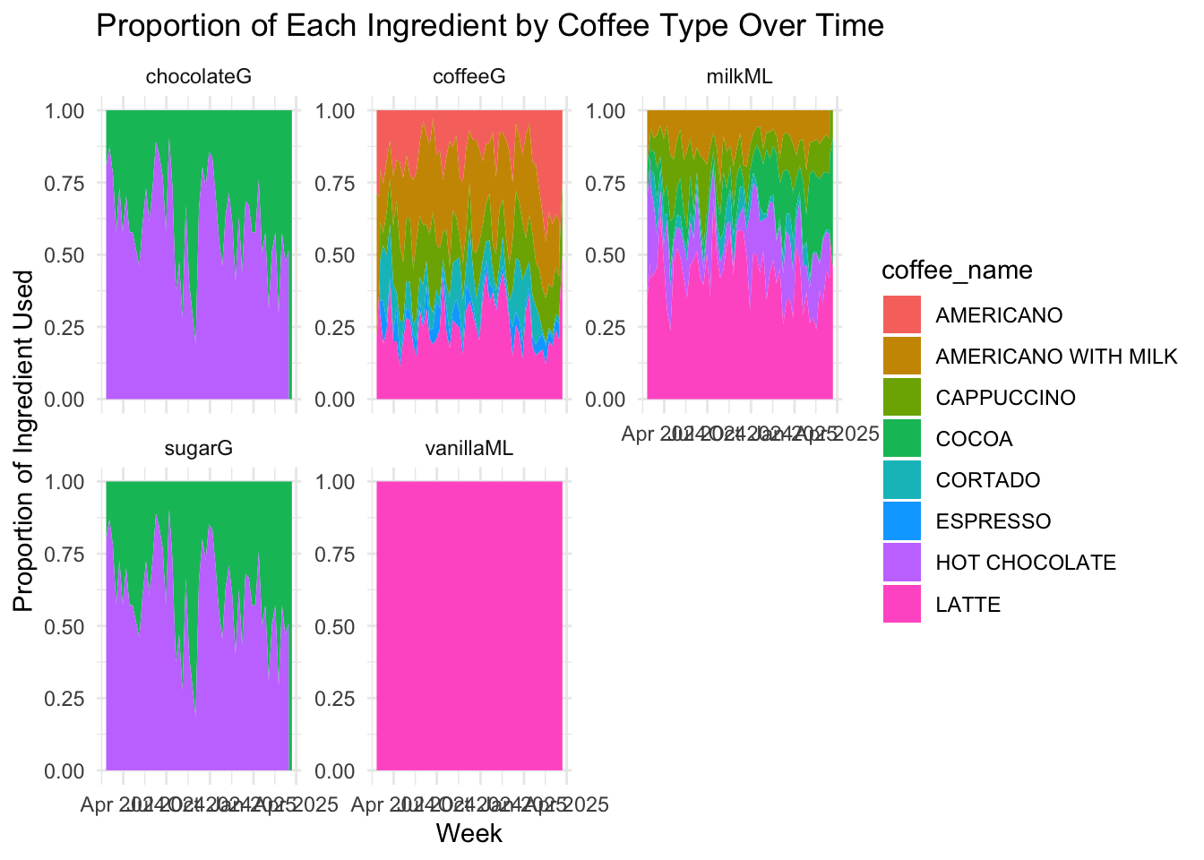

Appendix

Machine 1

Machine 1 Weekly ingredient demand vs. cups sold

References

Coffee Bros. 2024. “Milk-to-Espresso Ratio Calculator.” 2024. https://coffeebros.com/pages/milk-to-espresso-ratio-calculator.

Cordell, George. 2024. “Americano Coffee with Milk Recipe.” 2024. https://coffeelikers.com/americano-coffee-with-milk/.

Hersheyland Test Kitchen. 2025. “Hot Cocoa for One.” 2025. https://www.hersheyland.com/recipes/hot-cocoa-for-one.html.

Page, Amazon Product. 2025. “Torani Vanilla Syrup Pump – 8 Ml Per Pump.” 2025. https://www.amazon.com/dp/B09P49HWKK.

Raffii, Ahlam. 2024. “How to Make the Perfect Cappuccino.” 2024. https://www.thespruceeats.com/how-to-make-cappuccinos-766116.

Specialty Coffee Association. 2018. “Defining the Ever-Changing Espresso.” https://sca.coffee/sca-news/25-magazine/issue-3/defining-ever-changing-espresso-25-magazine-issue-3.

Wine Editors, Food &. 2025. “8 Types of Coffee Drinks to Order Around the World.” 2025. https://www.foodandwine.com/types-of-coffee-drinks-11724561.